This blog post showcases one way to download firm excess returns and characteristics from the BIGFI server and applies it in a simple investing context.
Requirements
- Jupyter Notebook + Python 3
- environment.txt file with credentials (provided by BIGFI or CBS Library)
- Code must be run at CBS or via a VPN to access the server
Download excess returns and trading signals
The code below downloads data from a BIGFI server and saves the data to data.csv (add to code – AS) in your current working directory.
The provided code also performs the following steps to prepare the data:
- Download data on excess returns and 3 characteristics for the US. The characteristics are: be_me, ret_12_1, market_equity. For more information on these, see JKP Docs.
- Include data between 2017-12-31 and 2022-12-31
- Exclude observations with missing market equity in month t and missing return in month t+1.
- Standardize the characteristics by subtracting the cross-sectional mean and dividing
by the standard deviation at each time. - Handle missing characteristics by replacing them with the cross-sectional (i.e. within
month) median, which is zero due to the previous step.
Jupyter Notebook
%pip install pandas python-dotenv sqlalchemy statsmodels matplotlibimport os
import pandas as pd
from dotenv import load_dotenv
from sqlalchemy import create_engine
import statsmodels.api as sm
import matplotlib.pyplot as plt
def download_data(query):
""" Download data from the database using a SQL query."""
# Load environment variables
load_dotenv('environment.txt')
try:
connection_string = (
f"mssql+pyodbc://{os.getenv('DB_USERNAME')}:{os.getenv('DB_PASSWORD')}@"
f"{os.getenv('DB_SERVER')}/{os.getenv('DB_NAME')}?"
f"driver=ODBC+Driver+18+for+SQL+Server&TrustServerCertificate=yes"
)
engine = create_engine(connection_string)
df = pd.read_sql(query, engine)
return df
except Exception as e:
print(f"Error: {e}")
return None
# Load data
query = f"""
select
id, date as eom, excntry, size_grp, me, ret_exc_lead1m,
be_me, ret_12_1, market_equity
from [{os.getenv('DB_SCHEMA')}].[{os.getenv('DB_TABLE')}]
where excntry='USA' and date >='2017-12-31' and date <'2022-12-31'
"""
df = download_data(query)
print(f"Data downloaded: {df.shape[0]} rows, {df.shape[1]} columns")
df.head(3)# Preprocess data
chars = [
'be_me', 'ret_12_1', 'market_equity'
]
df['eom'] = pd.to_datetime(df['eom'], format='%Y-%m-%d')
df['eom'] = df['eom'] + pd.offsets.MonthEnd(0) # end of month
df[chars] = df[chars].apply(pd.to_numeric, errors='coerce')
df[['me', 'ret_exc_lead1m']] = df[['me', 'ret_exc_lead1m']].apply(pd.to_numeric, errors='coerce')
# Restrict sample
df = df[df.me.notna()] #remove if no market cap
df = df[df.ret_exc_lead1m.notna()] # remove if no leading excess return
# fill missing values with XS median value and the standardise each month
for char in chars:
df[char] = df.groupby('eom')[char].transform(lambda x: x.fillna(x.median())) # Fill missing values with median
df[char] = df.groupby('eom')[char].transform(lambda x: (x - x.mean()) / x.std(ddof=0)) # Standardise
df[chars].describe().transpose()
df['ret_exc_lead1m'] = df['ret_exc_lead1m']*100 #scaling returns
df# Plotting the number of stocks in the cleaned sample
fig, ax = plt.subplots(figsize=(12, 6))
plt.plot(df.groupby('eom')['id'].count())
plt.title('Number of Stocks', fontsize=20)
plt.xlabel('Date', fontsize=16)
plt.ylabel('Count', fontsize=16)
plt.xticks(fontsize=12)
plt.yticks(fontsize=12)
plt.tight_layout()
plt.show()# Fit an OLS prediction model
Y = df['ret_exc_lead1m']
X = df[['be_me', 'ret_12_1', 'market_equity']]
# Fit OLS model
ols_model = sm.OLS(Y, sm.add_constant(X)).fit()
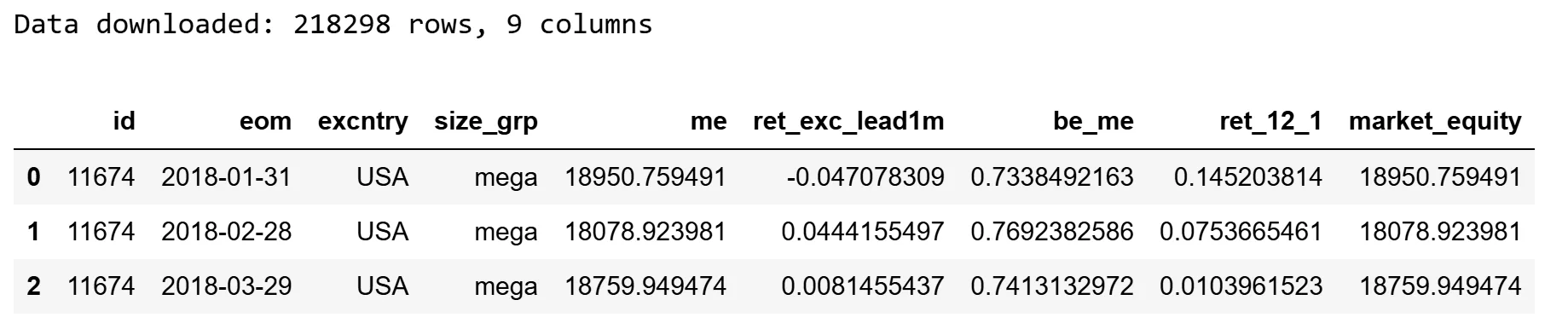
print(ols_model.summary())Let’s preview the data. We downloaded a firm-month panel with 218,298 rows and 9 columns containing information on stocks’ excess returns next month, their current book-to-market, their 1-year returns over the past year and their current market equity.
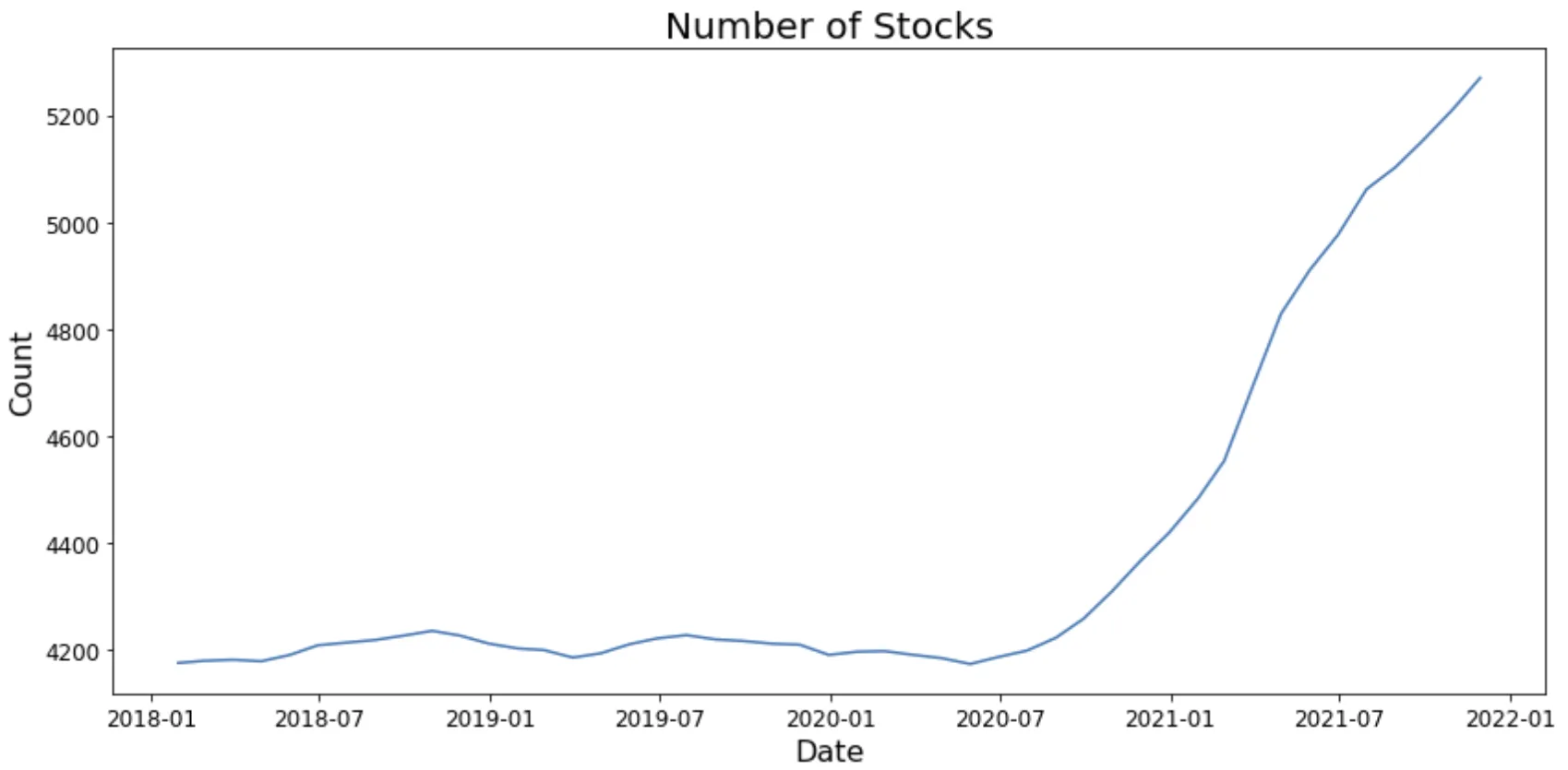
Now let’s plot the number of stocks we observe each month:

As seen in the plot, each month we start out with about 4200 stocks in the beginning of 2018 and then the number of stocks grows to about 5200 at the end in January 2022.
A simple model for investing
Let’s do a simple exercise where we train an OLS model to use the 3 characteristics to predict returns by fitting the following model
ret_exc_lead_1m = a + b * be_me + c * ret_12_1 + d * market_equity + error
Running that on the entire panel yields the following results:
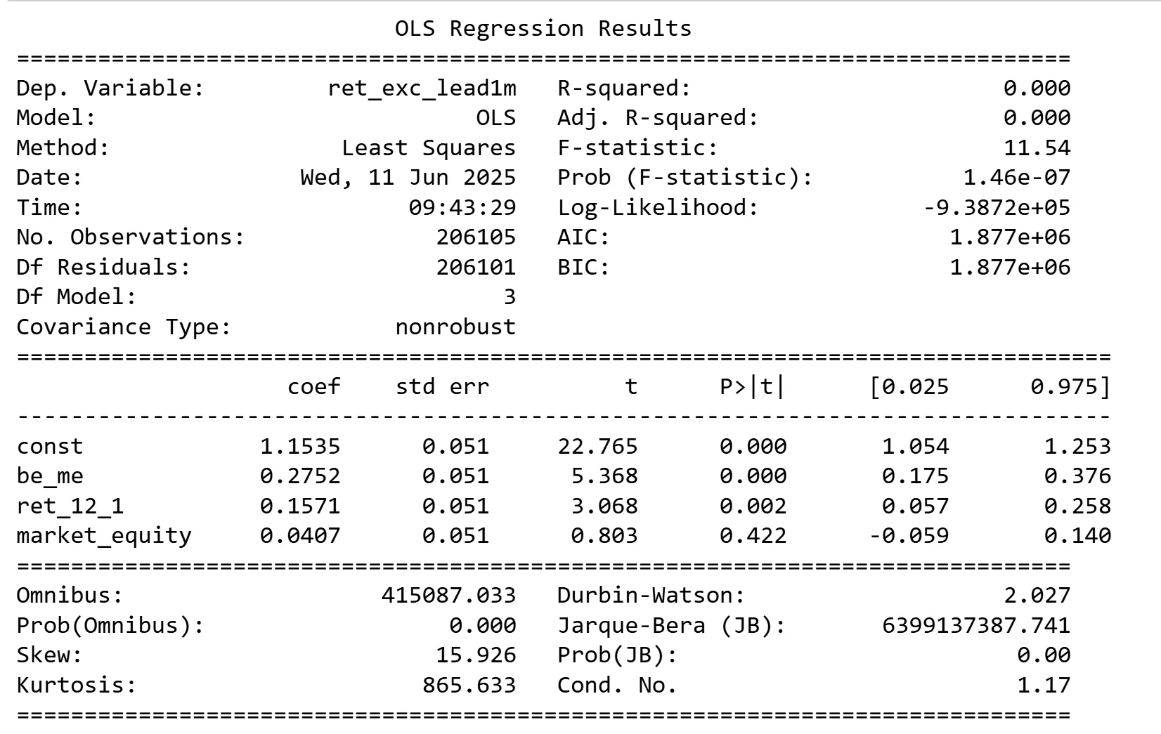
What is the trading strategy implied by this model? It is essentially a mix of Value, Momentum and Size strategies. Since it has a positive coefficient on all 3 characteristics this is a strategy that goes long cheap firms (low book-to-market), goes long on firms with high 1-year past returns and goes long firms with a large market equity consistent with Value, Momentum and Size strategies.